Histograma
Descripción
To launch the histogram dialog window, use the drop-down toolbar selecting the "Raster Layer" button on the left and "Histogram" in the drop-down button on the right. Make sure that the text box that displays the current layer is set to the name of the raster layer for which you want to see the histogram.

Histogram icon
The Histogram dialog shows a histogram of the statistical distribution of pixel values in the current view. This information is often useful when you are trying to color balance an image. In the middle of the dialog you will see the graph on which you can right-click to show a context menu with general options for this kind of graphics.
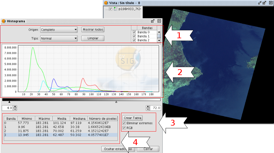
Histogram dialog window
In the upper part of the dialog (1) are the controls to configure the histogram:
1. Type of histogram
There are three types: "Normal", "Accumulated" and "Logarithmic".
- Normal: This is the normal histogram in which for every pixel value on the X axis the number of pixels is shown on the Y axis.
- Accumulated: Shows the accumulated number of pixels for every pixel value. The graph is therefore ascending.
- Logarithmic: Displays the histogram on a logarithmic Y axis, which may be useful for images that contain substantial areas of a constant value.
2. Data source
With this option you can select the data source for the histogram:
Current view (R,G,B):
With this option, the pixel values that are displayed in the current view of gvSIG will be used for the histogram. Therefore, the band selector shows only the R, G, and B values which are the visual bands. Every band will appear in its corresponding colour in the graph (red for R, green for G and blue for B). This is the default option when the histogram dialog is opened.
Complete histogram:
With this option, the histogram for the whole raster layer is calculated. Because of the amount of time that it would take to calculate the histogram for large images, the histogram is only calculated once and saved with a .rmf extension in the directory in which the image is stored. After the first time, the histogram for the same layer can be displayed much faster. (Keep in mind that if you delete the .rmf file that is stored with the image, you will lose its histogram information.)
3. Band selection
Apart from identifying to which band each histogram corresponds through its colour (in case of the current view Data Source) you can also identify the band by hovering the mouse over a point in the graph. The tooltip displays the band name and the value of the point.
Zoom operations
We can zoom in and out of the graph using the mouse.
- To zoom in on a part of the graph, draw a rectangle over it by pressing and dragging the mouse.
- To return to the original graph, click on the left mouse button on any point in the graph and drag to the left, then release the mouse button.
You can also zoom in and out using the context menu.
Context menu
When you right-click on any part of the graph, the context menu is shown with the following options:
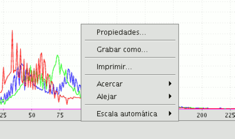
Histogram options. Context menu
- Properties: This will open the properties dialog of the graph, where you can configure characteristics such as the background colour, title, font etc.
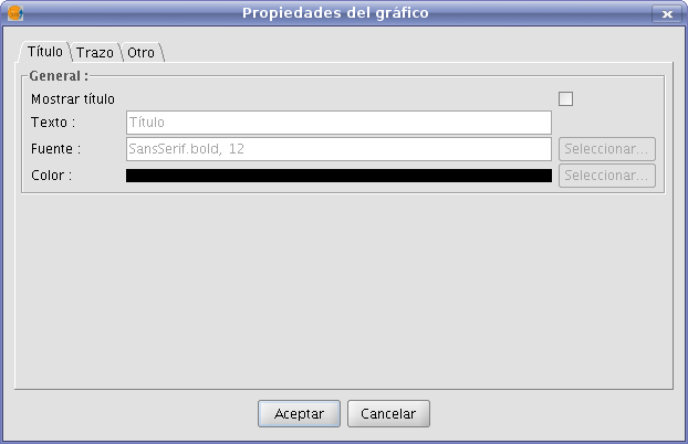
Histogram properties
- Save As: to save the graph as an image.
- Print: this opens the printer dialog from where you can print the graph.
- Zoom In: to zoom in on one or both of the axes.
- Zoom Out: to zoom out on one or both of the axes
- Auto Range: to adjust the zoom automatically to the window size, for one axis or for both.
5. Statistics (4)
The controls that appear under the graph allow the user to restrict the range of values (X axis of the histogram) on which the histogram is based. The default setting is the complete range so that, for example in a Byte data type image, the statistics are calculated for all the pixel values from 0 to 255. You can enter the values directly in the text boxes or use the + and – controls next to the text boxes. You can also slide the triangles over the sliding bar to select the range of values.

Sliding bar with pixel ranges
In this table, the statistics that correspond to the selected range of pixel values are shown in the text boxes. Each row of the table corresponds to one raster band as displayed in the histogram. The columns that are shown are:
- Minimum pixel value for the selected interval.
- Maximum pixel value for the selected interval.
- The mean (average) of all the pixel values for the selected interval in the histogram.
- Median pixel value for this interval.
- The number of pixels included in the selected interval.
6. Export the table (3)
You can export the table through the option "Save as DBF". The data contained in this table are the values of the current histogram. After creating the DBF table, it can be used as any other table in gvSIG.
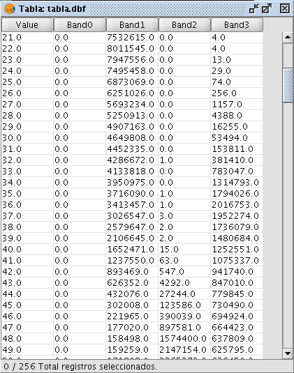
Resulting DBF table
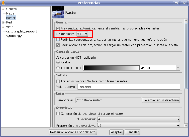
Preferencias
The Raster section of the Preferences dialog contains the option "Number of classes" where you can set the number of intervals in which the histogram is divided when the data type of the image is not Byte. For Byte images, this value is 256. In the preferences dialog, the default value of this option is 64 but you can choose any of the options (32, 64, 128, and 256). The intervals are the parts in which the range of values is divided. For example, if we have a DTM with values between 0 and 1 and there are 64 intervals, each interval will have a range of 1/64.
The number of classes does not only refer to histograms but also to other functionalities that require a division in intervals of value ranges.
Raster Preferences
